A machine that acts in the world must decide with evidence that is sometimes wrong. This unit shows how a joint probability distribution answers every question and why it is far too large to store, how a Bayesian network shrinks it with conditional independence, and how inference by enumeration and Bayes' theorem turn an observed effect into the probability of its cause. The naive Bayes spam filter and a Markov chain of the weather are worked through with every number, and a hidden Markov model infers rain from umbrellas.
Sample unit: the complete text
A robot’s distance sensor is right most of the time and wrong now and then, a cough is usually a cold and occasionally something worse, and the word “free” appears in most spam and in some perfectly ordinary mail. A machine that acts in the world must decide with evidence of this kind, and logic, which knows only true and false, cannot hold a belief that is 80 per cent sure. This unit shows how a machine keeps degrees of belief in many quantities at once without drowning in numbers, how it updates them when new evidence arrives, and how the same idea filters spam and follows the weather from day to day.
1 Degrees of belief and the joint distribution
Unit 1 introduced a probability as a number attached to an event; this unit reads it as a degree of belief. The two rules of Unit 1, the sum rule and the product rule, are all that is needed here, and the rest of this section is about one object that follows from them. The joint distribution of a set of random variables assigns a probability to every combination of values they can take together. For two yes-or-no variables that is a table of four numbers, and the numbers add up to one. To illustrate this, Table 1 gives the joint distribution of two variables of a doctor’s morning, whether a patient has influenza and whether the patient has a fever. The numbers are set by hand for this example and are reused in Section 2.
Fever
No Fever
Flu
0.0450
0.0050
No flu
0.0475
0.9025
Table 1. The joint distribution of the two variables flu and fever. Each cell is the probability that a patient has that combination, and the four cells add up to one.
The table is the complete description of the situation, because every question about the two variables can be answered from it with the two rules of Unit 1. The probability of a fever is the sum of the column, \(P(\mathrm{fever}) = 0.0450 + 0.0475 = 0.0925\), so that about 9 patients in 100 have one, and the probability of flu given a fever is the ratio
\[
P(\mathrm{flu} \mid \mathrm{fever}) = \frac{P(\mathrm{flu}, \mathrm{fever})}{P(\mathrm{fever})} = \frac{0.0450}{0.0925} = 0.486 ,
\]
so that about half of the patients with a fever have flu. Summing a row or a column is called marginalization, after the habit of writing the sums in the margin of the table, and dividing by the probability of what has been observed is conditioning. The whole of probabilistic reasoning consists of these two operations applied to a joint distribution, and the difficulty of the subject lies entirely in the size of that distribution.
The saving in the example comes from one idea, which is called conditional independence. Two variables \(A\) and \(B\) are conditionally independent given a third variable \(C\) when, once the value of \(C\) is known, learning \(B\) tells nothing more about \(A\). In the doctor’s morning, for example, once a cough is added to the flu and the fever of Table 1, a patient’s fever and cough are related, since both are more common with flu, but once the doctor knows that the patient has flu, the fever says nothing further about whether to expect a cough. The relation between fever and cough runs entirely through the flu.
The last sentence of the box deserves an example, because it is the point at which beginners most often go wrong. Over the summer, ice cream sales and the number of drownings at a beach rise and fall together, so the two are dependent, and someone who knew the day’s ice cream sales could guess the number of drownings better than someone who did not. Once the day’s temperature is known, however, the sales add nothing, because both numbers depend on the heat and on nothing else that links them. The two are conditionally independent given the temperature.
2 Bayesian networks
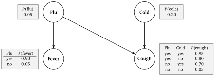
A Bayesian network writes the conditional independences of a situation as a drawing and the remaining dependences as small tables. It has one node for each random variable and an arrow from a node to every variable that depends directly on it. The nodes from which arrows arrive at a node are its parents, and the arrows may not form a cycle, so that one can never follow arrows from a node back to itself. Each node carries a conditional probability table, usually abbreviated to CPT, with one row for every combination of values of its parents and, in that row, the probability of each value of the node. A node without parents carries a plain probability. Figure 1 shows a network for the doctor’s morning with four variables, where influenza and a common cold are the two possible causes of the symptoms. The name of the structure goes back to a paper of 1985 by Judea Pearl of the University of California, Los Angeles, and his book Probabilistic Reasoning in Intelligent Systems, published in 1988, made the networks the standard tool for uncertain reasoning in artificial intelligence; he received the Turing Award for 2011 largely for this work.
Figure 1. A Bayesian network with four yes-or-no variables and its conditional probability tables. Flu and a cold have no parents and carry plain probabilities; fever depends on flu alone; cough depends on both. Each table lists the probability of “yes” for every combination of the parents’ values, and the probability of “no” is one minus that. The numbers are set by hand for this unit.
The tables in the figure hold \(1 + 1 + 2 + 4 = 8\) numbers. A joint table of four yes-or-no variables has \(2^{4} = 16\) cells and 15 free numbers, so even this small network nearly halves the count, and the saving grows with every variable that is added, as Section 1 showed for 30 of them. The absence of an arrow from cold to fever is the claim that a cold does not change the chance of a fever once flu is accounted for, and the absence of an arrow between flu and cold is the claim that catching one does not change the chance of catching the other. Arrows usually point from cause to effect, because then the tables are the ones a doctor can estimate, such as the probability of a fever given flu, but the mathematics does not require it; a network is a statement about which variables are conditionally independent of which, and nothing more.
The joint distribution of all the variables follows from the tables by a rule that Unit 1 used in its two-variable form. Applying the product rule repeatedly, one variable at a time, gives the chain rule of probability, and in a Bayesian network each factor of the chain simplifies, because a variable is conditionally independent of everything that is not its descendant once its parents are known. The descendants of a node are the nodes that can be reached from it by following arrows forwards.
For the network of Figure 1, the probability that a patient has flu, no cold, a fever, and a cough is \(P(\mathrm{flu})\,P(\text{no cold})\,P(\mathrm{fever} \mid \mathrm{flu})\,P(\mathrm{cough} \mid \mathrm{flu}, \text{no cold}) = 0.05 \times 0.8 \times 0.9 \times 0.8 = 0.0288\), which is one entry of the joint table, computed on demand from four small numbers. Any other entry is found the same way.
2.1 Inference by enumeration
A question put to a network has the form “what is the probability of this variable, given that I have observed those?” The observed variables are the evidence, the variable asked about is the query, and the remaining ones, which are neither, are hidden. The method that answers it directly from the factorization is called inference by enumeration and has four steps.
Write the joint probability of all variables as the product of the tables.
Put the observed values of the evidence into every factor.
For each value of the query variable, add up the product over every combination of values of the hidden variables, which is the marginalization of Section 1.
Divide each sum by the total of the sums, so that the results add up to one, which is the conditioning of Section 1.
Enumeration is exact, and for a network of a dozen variables it is quick. It fails for large networks for the same reason the joint table failed, since the sum in step 3 runs over every combination of the hidden variables, and twenty hidden yes-or-no variables mean \(2^{20}\) terms, about a million, for each value of the query. Cleverer exact methods reuse partial sums, but Gregory Cooper proved in 1990 that exact inference in a general network is NP-hard, which means that no known method is fast for every network, so large networks are answered approximately, by methods that draw random samples from the network and count; those methods lie beyond this unit.
3 Bayes’ theorem and the base rate
The commonest question put to a network has one cause and one observed effect, and for that case the enumeration of the last section collapses into a single formula, which Unit 1 introduced as Bayes’ rule and which is stated here in its general form with the names that every later unit uses.
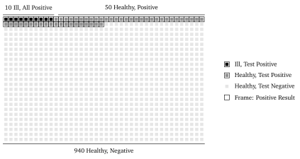
Unit 1 applied the theorem to a disease with a prevalence of 1 per cent, which means that one person in 100 has it, and to a test that is 95 per cent sensitive and 95 per cent specific. Sensitive means that the test is positive in 95 per cent of the ill, and specific means that it is negative in 95 per cent of the healthy. Unit 1 found that a positive result leaves the patient ill with a probability of only about 16 per cent. The result surprises almost everyone the first time, and the mistake behind the surprise has a name. The base rate fallacy is the habit of judging the evidence, a positive result from a good test, while forgetting the prior, which here is the prevalence, the base rate of the disease, and says that the disease is rare. Figure 2 shows the cure for the fallacy, which is to think in whole people instead of probabilities. Among 1,000 people, 10 have the disease and about 10 of them test positive, while 990 do not have it and about 50 of them test positive all the same. A positive result therefore comes from one of about 60 people, of whom 10 are ill, and \(10/60\) is the 16 per cent. Doctors and patients who are given the numbers in this form, as counts in a population, get the answer right far more often than those who are given percentages, a finding that Gerd Gigerenzer and colleagues established in a series of studies from the 1990s on.
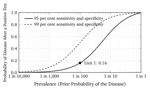
Figure 2. One thousand people, of whom 10 have the disease (dark) and 990 do not (light). The test marks about 10 of the ill and about 50 of the healthy as positive, drawn with a frame around them. Of the roughly 60 people with a positive result, 10 are ill, so a positive result means the disease with a probability of about 16 per cent. The counts of 9.5 and 49.5 are rounded to whole people.Figure 3. The probability of the disease after one positive result, plotted against the prevalence on a logarithmic axis, computed from Bayes’ theorem for a test with 95 per cent sensitivity and specificity (solid) and for one with 99 per cent of each (dashed). The dot marks the case of Unit 1.
The posterior depends on the prior as strongly as on the test. Figure 3 plots the probability of the disease after a positive result against the prevalence for the test above and for a much better one. At a prevalence of 1 in 10,000, as in screening a whole population for a rare condition, even the better test leaves a positive person healthy with a probability of 99 per cent. At a prevalence of 50 per cent, which is roughly the situation of a doctor who tests only patients whose symptoms already point to the disease, the same tests give posteriors of 95 and 99 per cent. The test has not changed; the prior has.
3.1 Two tests
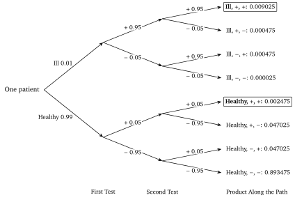
A second test is the natural next step, and the cleanest way to see what it does is to write Bayes’ theorem in terms of odds. The odds of a hypothesis are the ratio \(P(H)/P(\neg H)\), so that a probability of \(0.2\) is odds of \(0.2/0.8 = 1/4\), or \(1\) to \(4\), and the likelihood ratio of a piece of evidence is \(P(E \mid H)/P(E \mid \neg H)\), the factor by which the evidence is more probable if the hypothesis is true than if it is false.
Figure 4. The two-test case as a tree. Each branch carries its probability, each leaf the product along its path, and the posterior after two positive results is the share of the “ill” leaf among the two leaves with two positives, \(0.009025/(0.009025 + 0.002475) = 0.785\).
The independence in the example is a real condition, and in medicine it is often violated. If the two tests fail for the same reason, for instance because both detect the same substance and the patient’s body produces it for another reason, then the second positive adds much less than a factor of 19, and the honest posterior lies between 16 and 78 per cent. A Bayesian network with the two tests as children of the disease node states the independence explicitly, and a network with an extra arrow between the tests, or an extra common cause, states its violation.
Figure 5. Pierre-Simon Laplace as chancellor of the Senate, painted by Jean-Baptiste Paulin Guérin in 1838, after Laplace’s death. Credit: Jean-Baptiste Paulin Guérin, Wikimedia Commons, public domain.
4 The naive Bayes spam filter
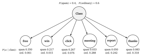
A spam filter has to decide, for each incoming email, between two values of one variable, which is its class, spam or ordinary mail. Its evidence is the email itself, represented in the way Unit 1 represented a sentence, as a list that says how often each word of a fixed vocabulary occurs in it. A Bayesian network for this has the class as the one parent and one child node for each word of the vocabulary, with an arrow from the class to every word and no arrows between the words, as Figure 6 shows for a vocabulary of six. The network is called the naive Bayes classifier, and the word “naive” refers to the missing arrows, which claim that the words of an email are conditionally independent of each other given its class.
Figure 6. The naive Bayes classifier as a Bayesian network. The class is the only parent; each word of the vocabulary is a child with no other parents, which is the claim that the words are conditionally independent given the class. The numbers are the smoothed probabilities of Table 2, as computed in the worked example.
The claim is false, since in real mail the word “free” makes “offer” far more likely in the same message, whatever the class. The classifier is nevertheless one of the most used in the history of the field, for two reasons. The first is that it needs so few numbers, two per word plus the prior, whereas a table of all the words together would need one per combination, so it can be estimated from a few hundred emails. The second is that it only has to rank the two classes, and the ranking is often right even when the probabilities behind it are badly off, because the errors of the independence assumption tend to inflate both scores by similar amounts.
4.1 Estimating the tables by counting
The tables of the classifier are not given by a doctor; they are estimated from a set of emails that someone has already sorted, which is the training set. The estimate is the one anyone would make. The prior \(P(\mathrm{spam})\) is the fraction of training emails that are spam, and the probability of a word given a class, \(P(w \mid c)\), is the number of times \(w\) occurs in the emails of class \(c\) divided by the total number of word occurrences in that class. Counting in this way is the same as choosing the numbers that make the training set as probable as possible, which statisticians call maximum likelihood estimation; Unit 4 turns the idea into the general recipe of learning, in which the parameters of any model are chosen to make a measure of error, called the loss, as small as possible.
Counting has one defect. A word that never occurred in the ordinary mail of the training set gets the probability zero, and the product rule then assigns probability zero to any ordinary email that contains it, whatever the other words say. One such word would override all the other evidence. The remedy is Laplace smoothing, which adds one to every count before dividing, as if every word had been seen once in each class, so that no probability is ever zero. In formulas, with \(V\) words in the vocabulary, the estimate of the probability of the word \(w\) in class \(c\) becomes \((n_{w,c} + 1)/(n_c + V)\), where \(n_{w,c}\) is the count of \(w\) in class \(c\) and \(n_c\) the total count of words in that class, and the \(V\) in the denominator keeps the probabilities of all words adding up to one, because the added ones, one for each of the \(V\) words, add \(V\) to the total count.
The decision then follows from Bayes’ theorem. The classifier computes, for each class, the prior multiplied by the probability of the words given the class, and chooses the larger. The probability of the evidence \(P(\text{email})\) is the same for both classes and need not be computed, which is why the rule below carries \(\arg\max\), the value of \(c\) for which the expression is largest, and no denominator.
The logarithms are a practical necessity rather than a decoration, and Unit 1 gave the reason. An email of 200 words contributes 200 factors, each around \(0.01\) or smaller, and a product of 200 factors of \(0.01\) is \(10^{-400}\), which a 32-bit or even a 64-bit floating point number cannot represent and rounds to zero. The logarithm of the same product is a sum of 200 ordinary negative numbers, about \(-900\), which any computer handles. Since the logarithm increases with the number it is applied to, the class with the larger product is also the class with the larger logarithm, and nothing is lost. To illustrate the whole method, Table 2 gives the counts of a training set of 20 emails made up for this unit, and the worked example classifies a new one.
Word
Count in 8 Spam Emails
Count in 12 Ordinary Emails
free
20
3
win
12
0
click
15
4
meeting
1
18
report
2
15
thanks
4
20
Total
54
60
Table 2. Word counts of a vocabulary of six words in a training set of 20 emails, 8 of them spam. Words outside the vocabulary are ignored. The counts were made up for this example.
Unit 5 returns to spam with logistic regression, which models \(P(c \mid \mathbf{x})\) directly instead of modelling the words given the class, and compares the two approaches; logistic regression usually wins once the training set is large, and naive Bayes usually wins while it is small.
5 Sequences and the Markov property
Many questions in artificial intelligence are about sequences, such as the weather on successive days, the words of a sentence, the positions of a robot, or the sounds of speech, and a network over a sequence of \(T\) days would need a node for every day and tables that grow with the length of the sequence. The way out is an assumption about time that Andrey Markov (1856-1922) introduced in 1906.
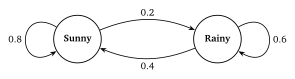
As a Bayesian network, a Markov chain is a row of nodes with one arrow from each day to the next and nothing else. Every node after the first has one parent and the same conditional probability table, which for \(k\) states is a \(k\) by \(k\) matrix called the transition matrix\(\mathbf{T}\), with the entry \(T_{ij}\) giving the probability of moving from state \(i\) to state \(j\) in one step. Each row of \(\mathbf{T}\) adds up to one, because the chain must go somewhere. Figure 7 draws a two-state chain for the weather, with states sunny and rainy, as a graph whose arrows carry the transition probabilities.
Figure 7. A two-state Markov chain for the weather. Each arrow carries the probability of the transition it shows, and the arrows leaving a state add up to one. The probabilities are set by hand for this unit.
The chain is run forward with a single multiplication. If the probabilities of the states on day \(t\) are written as a row vector \(\mathbf{p}_t = (P(\mathrm{sunny}), P(\mathrm{rainy}))\), then by the sum and product rules the probabilities on the next day are
\begin{equation}
\mathbf{p}_{t+1} = \mathbf{p}_t\,\mathbf{T} ,
\qquad\text{that is}\qquad
P(X_{t+1} = j) = \sum_{i} P(X_t = i)\,T_{ij} , \label{eq:step}
\end{equation}
which is the matrix-vector product of Unit 1 with the vector written as a row on the left, because the rows of \(\mathbf{T}\) are the starting states.
Markov first applied his chains to letters rather than weather. In a lecture to the Imperial Academy of Sciences in St Petersburg on 23 January 1913, he reported that he had gone through the first 20,000 letters of Pushkin’s verse novel Eugene Onegin, classified each as a vowel or a consonant, and counted the pairs. About 43 per cent of the letters were vowels, but a vowel followed a vowel only about 13 per cent of the time and followed a consonant about 66 per cent of the time, so the letters were not independent and a two-state chain described them well. A chain whose states are words rather than letters was for decades the standard model of language in speech recognition, and the probability that a modern language model assigns to the next word is a descendant of that idea, which lies beyond this unit.
5.1 Hidden Markov models
In the weather chain the state is observed every day. More often the state of interest cannot be seen directly, and what is seen is some noisy consequence of it. A speech recognizer, for example, does not hear the words, only the sound. A hidden Markov model is a Markov chain whose states \(X_t\) are hidden and which produces on each day an observation\(E_t\) with a probability \(P(E_t \mid X_t)\) that depends on the state of that day alone. As a Bayesian network it is the chain of the last section with one child hanging from each state node, and its tables are the transition matrix, the observation probabilities, and the distribution of the first state. The theory of these models was worked out in the 1960s by Leonard Baum (1931-2017) and colleagues at the Institute for Defense Analyses in Princeton, and from the 1970s to the 2010s they were the core of most speech recognizers.
The simplest question put to such a model is the probability of the hidden state today given all observations so far, and the answer is computed day by day by the forward algorithm, which repeats two steps. The first predicts the state of the next day from the current belief with Equation \eqref{eq:step}, and the second updates the prediction with the new observation by Bayes’ theorem, which multiplies each state’s probability by the probability of the observation given that state and then divides by the total.
Finding the single most probable sequence of hidden states for a whole series of observations, which a speech recognizer needs, is done by the Viterbi algorithm, and estimating the tables from observations alone by the Baum-Welch algorithm; both lie beyond this unit, as do sequence models whose state is a vector learned from data rather than a label chosen by hand.
6 Probabilistic reasoning today
The three ingredients of this unit, a factorized joint distribution, evidence entered into it, and Bayes’ theorem to turn the result round, are at work in systems in daily use. Bayesian networks have supported medical diagnosis since the late 1980s, when networks of hundreds and later thousands of nodes were built for pathology and internal medicine, and spam filters of the kind of Section 4 still run inside every large mail service. What has changed since the 1990s is where the tables come from. Here they were set by hand or counted from a small training set; Unit 4 replaces the counting by a general procedure that chooses the parameters of any model to make a loss as small as possible, and from Unit 6 on the models learned this way are neural networks, whose output probabilities are still read with the rules of this unit.
This is one of 16 units
Participants also get the quiz, the further reading, and the final exam.