

Search and Planning
A route planner, a puzzle solver, and a chess computer all describe their task as states, actions, and a goal, and then explore a tree of possibilities. This unit shows how breadth-first, uniform cost, and A* search organize that exploration, why the work grows as b to the power d, how an admissible heuristic tames it, and how minimax with alpha-beta pruning chooses a move. It ends with the numbers that explain why chess fell to search in 1997 and Go resisted until 2016.
A route planner that has never seen your town, a program that solves a sliding puzzle, and the computer that beat the world chess champion in 1997 all do the same thing. They describe their task as a set of states, a set of actions that lead from one state to another, and a goal, and they then explore the possibilities in an organized way until a path to the goal appears. This unit shows how that exploration is organized, why it becomes impossible as the number of steps grows, how a good estimate of the remaining distance tames that growth, and why the same ideas carried chess in 1997 but left Go out of reach for another nineteen years.
1 States, actions, and goals
Three ingredients turn a task into a search problem. The first is a description of the situation at any moment, the state, together with the initial state in which the task begins. The second is a set of actions, each of which changes one state into another, usually at some cost. The third is the goal, a condition that says which states count as finished. A solution is a sequence of actions that leads from the initial state to a goal state, and an optimal solution is a solution whose total cost is as small as possible.
The same three ingredients describe very different tasks. For example, when a route planner looks for the way from one town to another, a state is the town the traveller is in, an action is a road to a neighbouring town, the cost of the action is the length of the road, and the goal is the destination. In the 8-puzzle, eight numbered tiles slide in a 3 by 3 frame with one empty space (Figure 1). A state is the arrangement of the tiles, an action slides one of the tiles next to the empty space into it, every action costs one move, and the goal is the ordered arrangement. For a robot in a corridor, a state can be the robot’s position and the door it is facing, and the actions are the moves its motors can make.
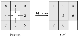
All the states that can be reached from the initial state, together with the actions that connect them, form the state space. For a map it is the map itself, and for the 8-puzzle it is a network of 181,440 arrangements, joined wherever a single move leads from one to the other, as Section 4 shows. The state space is given by the problem. The search tree is what a program builds while it explores that space. A tree in this sense is a drawing of circles joined by lines, in which each circle is called a node, the node at the top is the root, and the nodes hung directly below a node are its children. The root of the search tree is the initial state, and the children of a node are the states that one action reaches from it. Figure 2 shows such a tree in which every node has two children. The same state can appear in the tree more than once, because several sequences of actions may lead to it, so the tree can be far larger than the state space. A well written search keeps a list of the states it has already reached and does not grow a second branch for a state that another path finds again.
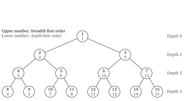
Every search algorithm of this unit follows the same loop. It keeps a collection of nodes that have been generated but not yet examined, called the frontier, which at the start holds only the root. In each round the algorithm takes one node from the frontier. If that node is a goal state, the search stops and the path from the root to the node is the solution. Otherwise the algorithm expands the node, which means that it generates the children by applying every possible action, adds to the frontier those children that have not been reached before, and starts the next round. The algorithms differ in a single decision, namely which node of the frontier to take next, and that one decision determines whether the search finds the shortest path, how much time it needs, and how much memory it fills.