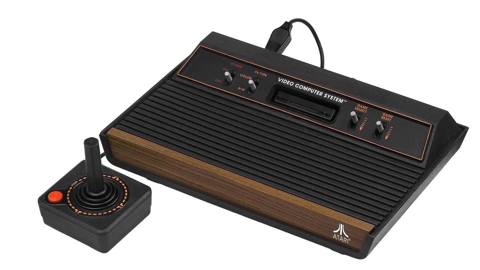
 Image: Evan-Amos, public domain
How many games does it take to learn Atari?
In February 2015 a paper in Nature reported a single learning system that had been set loose on 49 Atari 2600 games, from Breakout and Pong to Space Invaders and Seaquest, with the same network, the same settings, and no information about any game except the pixels on the screen, the score, and the eighteen positions of the joystick. On 29 of the games it played at or above the level of a professional human tester. On Breakout it had found the trick of tunnelling through the wall to bounce the ball behind it. And on every game it had practised for 50 million frames, which at the Atari's 60 frames a second is about 38 days of play without sleep.
What the network saw
The Atari screen is 210 by 160 pixels in 128 colours. The system, called the deep Q-network, or DQN, converted each frame to grey, shrank it to 84 by 84, and stacked the last four frames so that the network could see motion. Its input was therefore 84 by 84 by 4 numbers, about 28,000 of them. Three convolutional layers of the kind that read photographs turned those into features, and two fully connected layers turned the features into eighteen numbers, one per joystick action. The network had about 1.7 million parameters.
Each of the eighteen outputs was an estimate of a quantity called the action value, written \(Q(s, a)\): the total future score the agent expects if it takes action \(a\) in the current situation \(s\) and plays well afterwards, with scores in the far future discounted a little. Given these estimates, playing is easy: take the action with the largest \(Q\). Learning them is the whole problem.
Learning from one step at a time
Q-learning, an algorithm from 1989 by Chris Watkins, learns the action values from experience without a model of the game. After taking action \(a\) in situation \(s\), receiving reward \(r\), and arriving in situation \(s'\), it nudges its estimate towards the reward plus the discounted value of the best action from the new situation:
\[ Q(s, a) \leftarrow Q(s, a) + \alpha\left[r + \gamma \max_{a'} Q(s', a') - Q(s, a)\right]. \]The quantity in brackets is the difference between what the agent predicted and what it now, one step later, predicts; \(\alpha\) is a learning rate and \(\gamma\) the discount. With a small gridworld the estimates live in a table, and Unit 12 of the masterclass fills one by hand. An Atari screen has far too many possible situations for a table (even at four grey levels, \(4^{7056}\) of them), so DQN used the network as the table: the update became a gradient step on the network's weights towards the bracketed target.
Two devices made that stable, and both are in the paper's title of methods. Experience replay stored the last million transitions \((s, a, r, s')\) in a memory and trained on random batches from it rather than on the transitions as they happened, which broke the correlation between consecutive frames and let each experience be used many times. A target network, a copy of the network frozen for 10,000 steps at a time, supplied the \(\max Q(s', a')\) in the target, so that the network was not chasing a target that moved every time it moved. Without these, the same algorithm had diverged for years.
Thirty-eight days of practice
The number to carry away is the 50 million frames. The agent explored at first by choosing random actions and reduced the randomness over the first million frames, which is the exploration without which Q-learning finds nothing. The reward it saw was clipped to \(+1\), \(0\), or \(-1\) so that one set of settings could work across games whose scores differ by factors of a thousand. And it had no idea of a ball, a paddle, or a wall. Every regularity it exploited it had to find from the pixels by trial, which is why it needed about a thousand times more play than a person who starts with those concepts in hand.
The deep Q-network could also fail in a way a person would not. In Montezuma's Revenge, a game whose first reward is many steps from the start and requires a sequence of unrewarded actions, it scored zero. Random exploration never stumbled on the first reward, so there was nothing to learn from. Games that need planning across a long horizon were hard for the same reason; the 29 games it mastered were those in which rewards come quickly and often.
Why robots cannot do this
Fifty million frames cost nothing on an emulator; the games ran faster than real time on a single computer and the agent never broke anything. A robot that learns to pick up objects moves at real speed, wears its joints, and can drop the object on the floor. A million grasps is a year of continuous operation. A self-driving car cannot explore by random actions at all. Learning from so little experience that it could be collected in the physical world is called sample efficiency, and it is the gap between the Atari result and the robot that is still not in your house.
The responses to the gap are the active directions of the field. Learning a model of the world so that the agent can practise in imagination, as a later system from the same laboratory did for Atari with far fewer frames. Simulating the robot and transferring the learned policy to the real one, with randomized physics so that the policy does not overfit to the simulator. Learning from demonstrations before reinforcement begins, which is how a language model is first taught to answer before human preferences are used to refine it. Each of these borrows from the method of 2015 and tries to pay less for it.
The paper, "Human-level control through deep reinforcement learning" by Volodymyr Mnih and colleagues at DeepMind, is at the journal, with the 49 scores in its figure 3. Unit 12 of the AI Masterclass works four Q-learning updates on a gridworld with the numbers, explains what the deep Q-network changed and why, and goes on to policy gradients, AlphaGo, and the robot of Pieter Abbeel's group that learned to screw on a bottle cap from camera pixels.