

Neural Networks and Backpropagation
A single neuron can draw one straight line through its data, and the XOR function shows why that is not enough. This unit puts neurons in layers, computes XOR with three of them, and derives backpropagation, the algorithm that finds the gradient of every weight in one backward sweep, on a network small enough to train by hand. It ends with the softmax output for many categories, a two-layer network that reads handwritten digits with 98 per cent accuracy, and what the universal approximation theorem does and does not promise.
The classifier of Unit 5 was one neuron. It took a weighted sum of its inputs and squeezed the result through a sigmoid, and a single neuron of this kind can only draw one straight line through its data. This unit puts neurons behind one another, so that the output of one is the input of the next, and shows that two layers of them can compute what one cannot. The price is that the weights deep inside the network no longer have a closed formula of the kind Unit 4 found for linear regression, and not even an obvious gradient. The method that finds every gradient in one backward sweep, backpropagation, is the subject of the middle of the unit and is carried out by hand on a network small enough to fit on one page.
1 The artificial neuron
A real neuron receives signals from thousands of other neurons through its dendrites, and when the combined excitation is strong enough it fires an electrical pulse down its axon. Warren McCulloch (1898-1969) and Walter Pitts (1923-1969) proposed in 1943 that this could be described as a logical device: a cell that adds up its inputs and switches on when the sum passes a threshold. The human brain has about 86 billion such cells, and the retina is built from the same kind of cell; the plate at the head of this unit shows the cells of the retina as Santiago Ramón y Cajal (1852-1934) drew them. The artificial neuron of this unit keeps only the arithmetic of this picture. It takes the dot product of Unit 1, adds a constant, and passes the result through a fixed function.
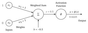
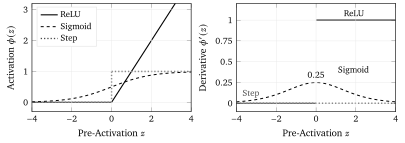
The weighted sum \(z\) is called the pre-activation, and the output \(a\) the activation. The bias \(b\) plays the part of the threshold: with \(b = -\theta\) the neuron switches on when \(\mathbf{w}\cdot\mathbf{x}\) exceeds \(\theta\). Figure 1 draws the whole device for two inputs. The activation function \(\phi\) is the only nonlinear step, and three choices account for almost everything in this unit (Figure 2).
- The Heaviside step function, \(\phi(z) = 1\) for \(z > 0\) and \(0\) otherwise, is the switch of McCulloch and Pitts and of the perceptron of Section 2. Its derivative is zero everywhere except at the jump, so a gradient cannot pass through it.
- The sigmoid, \(\sigma(z) = 1/(1 + e^{-z})\), is a smoothed step that runs from 0 to 1 and equals \(0.5\) at \(z = 0\). Unit 5 used it to turn a score into a probability. Its derivative has the convenient form \(\sigma'(z) = \sigma(z)\,(1 - \sigma(z))\), which is at most \(0.25\), at \(z = 0\).
- The ReLU function, \(\mathrm{ReLU}(z) = \max(0, z)\), takes its name from the field’s term rectified linear unit; this masterclass says the ReLU function throughout. It passes positive inputs unchanged and sets negative ones to zero. Its derivative is 1 for \(z > 0\) and 0 for \(z < 0\), and it is the usual choice in the hidden layers of large networks today, for reasons Unit 7 gives; the largest language models use smoothed variants of it, which go beyond the unit.
With the sigmoid as \(\phi\), the neuron is exactly the logistic regression of Unit 5, which read its output as the probability \(P(y = 1 \mid \mathbf{x})\). Everything that unit did with one neuron, the cross-entropy loss and the gradient step, carries over to the neurons of this unit. What is new is what happens when neurons feed one another.