

Classifiers and Decision Trees
Three classifiers built by hand on real data: logistic regression with the cross-entropy loss derived from maximum likelihood, k-nearest neighbours, and decision trees grown with entropy and information gain, with random forests as the step beyond one tree. The unit ends with the measures that tell you how good a classifier really is, the confusion matrix, precision and recall, and the ROC curve, and with the debate about readable models in high-stakes decisions.
A spam filter, a bank’s fraud detector, and a program that reads chest X-rays all answer a question of the same shape, namely to which of a few categories a given input belongs. Unit 4 fitted a straight line to numbers that could take any value, but a label that is either 0 or 1 needs a different model, a different loss, and above all a different way of judging the result, because a classifier that is right 98 per cent of the time can still be useless. This unit builds three classifiers that work in different ways, namely logistic regression, nearest neighbours, and decision trees, and it ends with the measures that say how good a classifier really is.
1 Logistic regression
Classification is the task of predicting a category rather than a number. When there are two categories the task is called binary classification, and the labels are written \(y = 1\) for the category of interest (spam, ill, Iris virginica) and \(y = 0\) for the other. The input is a vector \(\mathbf{x}\) of \(d\) features, as in Unit 1, and the training set holds \(N\) labelled examples \((\mathbf{x}_i, y_i)\), as in Unit 4.
1.1 Why a straight line is the wrong model
Unit 4 fitted the line \(\hat{y} = \mathbf{w}\cdot\mathbf{x} + b\) to its data by least squares, and one could try the same with labels of 0 and 1. The result is poor for two reasons. A line that passes through 0 and 1 keeps going, so the model predicts \(1.7\) for an input far on one side and \(-0.4\) for an input far on the other, and neither number means anything as a label. The second reason is worse. The squared error punishes a prediction of \(2.3\) for a flower whose label is 1 as heavily as a prediction of \(-0.3\), because both are \(1.3\) away from the label, although the first flower is on the correct side by a wide margin and the second is on the wrong side.
Both problems disappear when the weighted sum is passed through a function that squeezes every number into the interval from 0 to 1. The function the field uses is the sigmoid, \begin{equation} \sigma(z) = \frac{1}{1 + e^{-z}} , \label{eq:sigmoid} \end{equation} drawn in Figure 1. It rises from 0 for large negative \(z\) to 1 for large positive \(z\), passes through \(\sigma(0) = 0.5\), and is symmetric in the sense that \(\sigma(-z) = 1 - \sigma(z)\). Unit 1 met it as the derivative of \(\log(1 + e^z)\); that derivative, \(e^z/(1 + e^z)\), is the sigmoid written in another form. Its own derivative has a form that the loss of Section 1.2 will make use of, \begin{equation} \sigma'(z) = \sigma(z)\,\bigl(1 - \sigma(z)\bigr) , \label{eq:sigmoidprime} \end{equation} which follows from the chain rule of Unit 1 applied to \((1 + e^{-z})^{-1}\). The curve is also called the logistic function, a name given by the Belgian mathematician Pierre François Verhulst (1804-1849), who introduced it in 1838 to describe how a population grows quickly at first and then levels off, and who gave it the name in 1845.
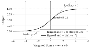
The output is a probability, which is what makes the model useful beyond the bare decision. A hospital can treat a patient with \(P = 0.95\) differently from one with \(P = 0.55\), although both lie on the same side of the threshold. The weighted sum \(z = \mathbf{w}\cdot\mathbf{x} + b\) has a meaning of its own. Solving Equation \eqref{eq:sigmoid} for \(z\) gives \(z = \log\bigl(P/(1 - P)\bigr)\), the logarithm of the odds \(P/(1 - P)\) that Unit 3 defined, so that each increase of \(z\) by one multiplies the odds in favour of \(y = 1\) by \(e \approx 2.72\). This is why a weight \(w_j\) is read as the change in the log-odds for a change of one in the feature \(x_j\), and why the model is called a regression although it classifies, because it fits a straight line, as Unit 4 did, to the log-odds instead of to the label.