

Attention and Transformers
In 2014 a decoder was first allowed to look back at every word of the sentence it was translating, with weights it had learned, and in 2017 eight researchers kept only this looking back and dropped the recurrence. This unit works one step of scaled dot-product attention by hand on three tokens, shows why the scores are divided by the square root of the key dimension, adds heads and positional encodings, and assembles the transformer block. It counts the 65 million parameters of the original model, explains why the architecture trains so fast and why its cost grows with the square of the text length, and ends with BERT, GPT, and the vision transformer as three uses of one block.
Unit 10 ended at a bottleneck. An encoder read a whole sentence and pressed it into one vector, and the decoder had to write the translation from that vector alone, however long the sentence was. This unit follows the idea that removed the bottleneck in 2014, which lets the decoder look back at every word of the source sentence with weights it has learned. It then turns to the architecture of 2017, which kept only this looking back, dropped the recurrence, and is now underneath the large language models and much of computer vision. By the end the reader will have computed one step of attention by hand, counted the parameters of the original transformer, and seen why the work it does on a long text grows with the square of the text’s length.
1 Looking back at the source
The encoder-decoder model of Unit 10 translates in two stages. A recurrent encoder reads the source words \(x_1, \ldots, x_T\) and produces one hidden state \(\mathbf{h}_j\) after each word, and a recurrent decoder starts from the last of these states and emits the target words one at a time. Everything the decoder knows about the source must pass through that last state, which is a vector of a few hundred or a few thousand numbers, and a sentence of forty words does not fit into it well. In experiments of 2014 the translation quality of such models fell steeply once sentences grew longer than about twenty words.
In September 2014 Dzmitry Bahdanau, Kyunghyun Cho, and Yoshua Bengio of the Université de Montréal posted a paper that removed this bottleneck. Their decoder keeps all encoder states and, before it emits the \(i\)-th target word, computes a separate context vector for that word, which is the vector the decoder reads the source from while it writes that word. A small network \(a\) gives every encoder state \(\mathbf{h}_j\) a score \(e_{ij}\) by comparing it with the decoder’s own previous state \(\mathbf{s}_{i-1}\), the scores are turned into weights \(\alpha_{ij}\) that sum to one, and the context vector \(\mathbf{c}_i\) is the weighted sum of the encoder states, \begin{equation} e_{ij} = a(\mathbf{s}_{i-1}, \mathbf{h}_j), \qquad \alpha_{ij} = \frac{e^{e_{ij}}}{\sum_{k=1}^{T} e^{e_{ik}}}, \qquad \mathbf{c}_i = \sum_{j=1}^{T} \alpha_{ij}\,\mathbf{h}_j . \label{eq:bahdanau} \end{equation} The function \(a\) was a feed-forward network with one hidden layer, trained together with everything else by backpropagation (Unit 6). The weights \(\alpha_{ij}\) are the output of a softmax, which Unit 6 introduced for the output layer of a classifier, and here it plays a different part: it decides how much of each source word reaches the decoder at this step. The paper called the weights a soft alignment, because they say which source words the \(i\)-th target word is translated from, and the field soon called the whole mechanism attention. Figure 1 shows the arrangement at the step that produces the second target word.
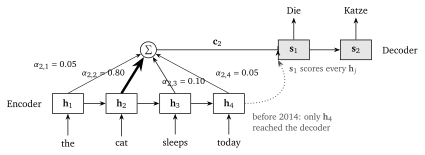
The gain was measured on the translation task of the 2014 Workshop on Machine Translation from English to French. The model with attention kept its quality on sentences of fifty words, where the model without it had lost a large part of its score, and it came close to the best translation system of the time, which was not a neural network but a statistical system built from tables of matching phrases. The alignments it learned could be drawn as a grid of the weights \(\alpha_{ij}\), and they showed the model putting the French adjective after its noun, which is the reverse of the English order, without having been told that French does this. The scoring network \(a\) was soon replaced by something simpler, because in 2015 Minh-Thang Luong, Hieu Pham, and Christopher D. Manning at Stanford showed that the plain dot product of the two vectors, \(\mathbf{s}_{i-1}\cdot\mathbf{h}_j\), works as a score. That is the form the rest of this unit uses.