

Pretraining and Scaling Laws
Every assistant began as a model trained to predict the next token of a large part of the written internet. This unit works out what that model learns and which loss it minimizes, how byte pair encoding turns text into tokens and why some languages cost six times more of them, where the data come from and who filters them, and how many floating point operations and megawatt-hours a run like GPT-3 took. It then presents the scaling laws of 2020 and the Chinchilla result of 2022, with a worked compute-optimal model, and ends with few-shot prompting, the debate about emergent abilities, and what a benchmark score does and does not say.
Every assistant that answers in fluent sentences began as a model that did one thing: it read text and guessed the next piece. Units 10 and 11 built the machinery, which consists of the token, the embedding, the attention block, and the transformer. This unit is about what happens when that machinery is trained on a large part of the written internet, how many floating point operations and how much electricity that takes, and the measured laws that say how the result improves when the model, the data, and the computing budget grow. It ends where Unit 14 begins, with a model that predicts text very well and is not yet an assistant.
1 Next-token prediction
A language model assigns a probability to every sequence of tokens. Unit 10 defined a token as the piece of text a model reads at one step and introduced the probability of a sequence as a product of conditional probabilities, one for each token given all the tokens before it. For a text \(w_1, w_2, \ldots, w_T\) this reads \begin{equation} p_{\boldsymbol{\theta}}(w_1, \ldots, w_T) = \prod_{t=1}^{T} p_{\boldsymbol{\theta}}(w_t \mid w_{<t}) , \label{eq:chain} \end{equation} where \(w_{<t}\) stands for the tokens \(w_1\) to \(w_{t-1}\) and \(\boldsymbol{\theta}\) for all parameters of the model. The factorization is the chain rule of probability from Unit 3 and holds for any distribution, so it involves no approximation. What the transformer of Unit 11 computes at position \(t\) is one such factor, \(p_{\boldsymbol{\theta}}(w_t \mid w_{<t})\), as a softmax over \(V\) scores, one for each token of the vocabulary, where \(V\) is the size of the vocabulary. Figure 1 shows what such a distribution looks like for one context.
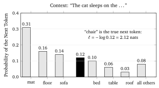
Pretraining is the training of this model on a very large body of ordinary text, with no labels except the text itself. Each position supplies one training example: the context \(w_{<t}\) is the input and the token that actually followed, \(w_t\), is the class label. The loss is the cross-entropy of Unit 5. There it compared a predicted probability with a label from two or ten categories; here it compares the predicted probability with a label from \(V\) categories, and \(V\) is typically between 30,000 and 200,000.
Two readings of this number give a feeling for its size. First, the loss is the logarithm of the perplexity that Unit 10 defined, so a loss of \(2.0\) nats per token is a perplexity of \(e^{2.0} = 7.4\), as if the model were choosing uniformly among about seven tokens at every step. Second, the loss in bits is the average number of bits that an ideal compressor built from the model would need per token, because a token that the model expects with probability \(p\) can be written down in about \(-\log_2 p\) bits, few for a likely token and many for a surprising one. For example, a token with probability \(1/2\) costs one bit and a token with probability \(1/1024\) costs ten. This is why the people who train these models speak of “bits per token” and of compression together.
From here on the unit uses \(N\) for the number of parameters of a model and \(D\) for the number of tokens it is trained on, as the scaling literature does. Units 1 to 12 used \(N\) for the number of training examples, and that meaning does not return in this masterclass.